Lab scheduling software is the unsung hero of lab automation.
An unscheduled lab workflow isn’t just inefficient—it’s often impossible to execute—leading to a frustrating barrier in protocol development. If you’re responsible for an automation system, your scheduler is what turns an abstract workflow into actual productivity. But while scientists talk about “lab scheduling,” they frequently mean very different things. That’s because not all schedulers are built the same, and the term itself has become overloaded with assumptions.
In this article, we’ll clarify the meaning and mechanics of lab scheduling, survey different approaches, and illustrate why modern scheduling—especially when paired with powerful solving tools—represents a significant leap forward. We also want to explain what laboratory scheduling software looks like from Automata’s point of view, explore the different approaches labs are using today, to show how modern scheduling—especially when powered by smart solvers—is transforming lab operations from the ground up
As lab scheduling continues to quickly evolve, understanding the approaches and trade-offs of different systems will help you make better choices to integrate into your whole automation stack.
What is a Lab Scheduler?
Before we can discuss what lab scheduling is, we first need to introduce the concept of a workflow.A “workflow” in the context of an automated lab typically describes a series of steps, or tasks, each generally associated with a specific instrument. Each task—e.g. “wash plate,” “spin plate,” “seal microplate,” “peel microplate”—is connected to others by dependencies (which tasks must finish before others can start) and constraints (how long tasks can wait, maximum times out of incubator, etc.). When the list of tasks is articulated with all of these constraints, we have a directed graph of tasks. In a very literal sense, this is the workflow
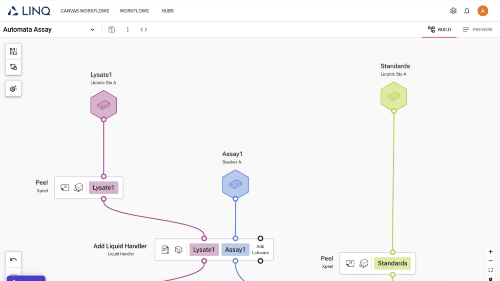
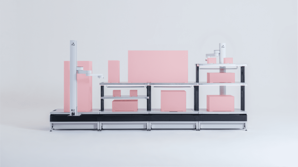
We’ll focus on a workflow as this top-level articulation of the task graph. We’ll omit discussion of transport times or computation of what robotic transport methods are available. Our platform LINQ abstracts these away from the end user – transport and robot movements happen under the hood.
However, a mere graph of tasks isn’t enough to actually run a workflow. You need a schedule, i.e. a plan that maps tasks onto a timeline with specific allocations to instruments. This ensures constraints are observed, conflicts are avoided, and instrument utilization and throughput is high.
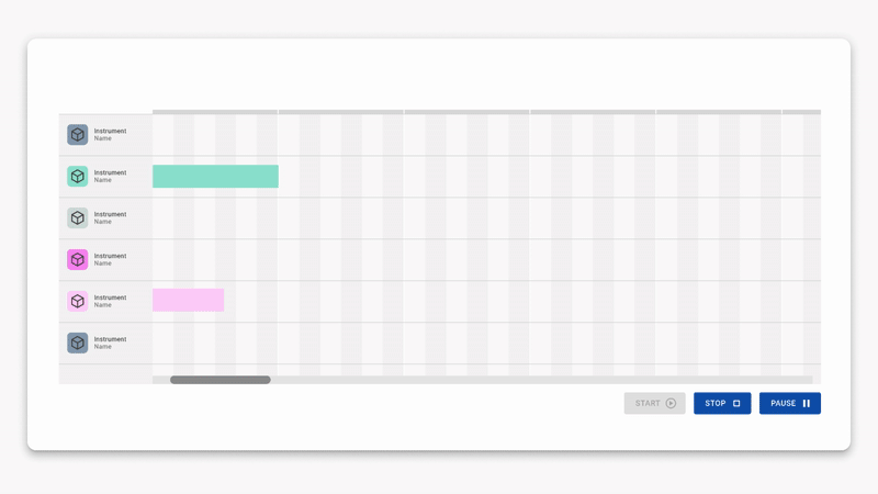
The workflow graph can be visualized as a flow chart with constraints, and the workflow schedule (sometimes plan) can be visualized as a Gantt chart or similar timeline view
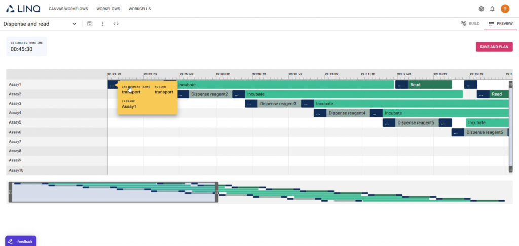
Creating this schedule is a non-trivial problem—commonly referred to as a combinatorial optimization problem—since multiple tasks may run in parallel, and numerous resources, timinsg, and ordering constraints must be considered. The core discussion at hand here is how schedulers get to a solution.
It can’t be overstated how computationally complex this “flexible job shop scheduling” problem can be, and it’s this complexity that leads to different approaches to scheduling—that’s why we have an entire team of devs dedicated to our scheduler here at Automata!
Dynamic vs. Static Lab Schedulers
If solving a lab schedule is so difficult, why not simply avoid the problem altogether? Instead of generating a plan upfront (static scheduling), you could opt for a dynamic approach, and just fulfill every task on the fly (dynamic scheduling).
- A static lab scheduler, in contrast, uses a solver or algorithm to produce an optimized sequence of tasks before the run starts. All tasks are assigned to resources along a timeline in an effort to respect constraints and minimize total makespan or other relevant performance metrics.
- A dynamic lab scheduler operates in a loop, continuously scanning for tasks that are ready to execute and assigning them to available instruments in real time. It makes immediate decisions rather than attempting to solve the entire workflow plan in advance.
Problems with Dynamic Lab Schedulers
While dynamic scheduling can be computationally simpler (no heavy-duty solver is required) it introduces several serious issues:
- Deadlocks
In certain conditions (e.g., limited resource availability, circular dependencies), a dynamic scheduler can get “stuck” if tasks wait on each other in a cycle. For example, imagine two robotic arms each holding microplates that the other arm needs in order to proceed. Without a global plan, this can halt the entire workflow. These deadlocks are no doubt a familiar and frustrating experience for many readers. - Suboptimal or Random Efficiency
Dynamic schedulers typically only look at immediate availability of instruments. They don’t attempt to optimize the overall timeline. As a result, they may produce a suboptimal schedule that inflates the total run time or underutilizes expensive lab equipment. In fact, in even a moderately complex workflow, in our experience, it is almost guaranteed that a dynamic scheduler will struggle to optimize utilization. - Difficult Constraint Enforcement
Ensuring tight timing constraints (e.g., do not exceed 2 minutes out of the incubator) is non-trivial in a purely reactive system. One must rely on heuristics or guardrails that often fall short if unanticipated variations occur. Failing that, a workflow will need to be simulated in detail to ensure constraints can be met, there is no other way of knowing without a static solution.
Simulation and Dynamic Lab Scheduling
To mitigate these issues, every dynamic scheduler we’ve encountered on the market allows for simulation. An initial task graph can be created, and then simulated based on estimated time required for each task. If issues are encountered, initial conditions, instrument allocation or other tweaks can be made to resolve the issue (e.g. a deadlock). This goes on and on in a loop until a sequence that “works” can be found. However, as you can imagine, this can be an arduous and frustrating process, where tweaking starting parameters can be opaque relative to the outcome they might have on the workflow.
To make matters more difficult, time estimates rarely fit reality. In fact, even for relatively timing-consistent actions, small deviations accumulate. This isn’t even to mention the challenge of working with unpredictable timings, for example tasks which may involve a human operator. All of this together can accumulate, revealing new deadlocks or constraint violations that are only discoverable when a workflow first goes live on hardware.
These are the worst kinds of lab scheduling issues: failed runs can waste reagents and reduce throughput, undermining the very rationale for lab automation.
Problems with Static Lab Schedulers
Static lab scheduling avoids many of these pitfalls. By solving globally from the outset, it can:
- Eliminate deadlocks, since constraints are modeled in the solver. In fact, deadlocks are impossible with a static solve: by definition a deadlocked state implies no solve.
- Respect complex timing constraints, scientific limits, and resource sharing rules.
- Often yield schedules that are close to optimal. Of course it’s mathematically impossible to ensure you’ve found the most optimal solution. Perhaps quantum computers will help here…
However, you may have already noticed the major problem here: if the issue with dynamic schedulers and simulation is the accumulation of difference between timing estimates and real-life execution, aren’t static schedulers even more prone to this issue? In other words, if actual run times deviate substantially from the predicted times, the schedule’s validity is at risk. In a busy lab, things happen—delays, instrument faults, unexpected reagent prep times. A static approach can’t automatically adapt unless it re-solves the entire plan. And re-solving can introduce delays that derail utilization, or simply be computationally infeasible. A workflow can’t stop for ten minutes to resolve!

For many with experience with purely static schedulers, this single pitfall is enough to make any static scheduling approach infeasible. So why does Automata choose static scheduling?
Dynamic Replanning Static Scheduling
This is where modern constraint solvers—such as Google’s OR-Tools—offer a major advantage. OR-Tools is an open-source suite providing mixed-integer programming, constraint programming, and specialized solvers (like the CP-SAT solver) to handle complex scheduling scenarios.
In a “dynamic replanning” model, you keep the benefits of a static solver (full awareness of constraints, near-optimal scheduling) but allow the solver to re-run when real-world events deviate from the plan. OR-Tools supports fast re-solving by taking the prior schedule as a hint—akin to how Google Maps quickly recalculates a route if you miss a turn. Instead of starting from scratch, the solver uses the old solution to guide the new one. This incremental approach can bring re-solve times down to fractions of a second, even when an initial solve may have taken dozens of minutes, making it viable for real-time or near-real-time corrections.
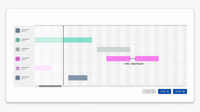
For instance, imagine a microplate sealer runs slower than predicted. The scheduler detects a delay, updates the known run time, and triggers a re-solve. If we think intuitively, like a human and not like a computer, this can be mathematically easy. We shift all uncompleted bars on the Gantt chart forward, and take a look at time constraints to see if they are still respected. In a similar, but much more mathematically complex way, OR-Tools reuses much of its previous solve on every resolve. The workflow can keep moving without lengthy downtime or the risk of constraints being violated due to out-of-date plans.
In this way, a Dynamic Replanning Static Scheduler can enjoy the power of static scheduling, the flexibility of dynamic scheduling, and even still be less vulnerable to deviations from estimates yielding unexpected workflow graph violations only discoverable at runtime.
Types of schedulers: Dynamic vs. Static vs. Static Replanning
Taken together, we can classify laboratory scheduling approaches in three main categories:
- Dynamic (Reactive) Scheduling: No global plan, purely local decisions. Avoids solver overhead but brings exposure to deadlocks and suboptimal utilization.
- Static Scheduling: Pre-computed, globally optimized plan. Excellent for ensuring constraints and resource usage, but deeply vulnerable to unexpected variations during execution.
- Static Scheduling with Dynamic Replanning: Combines the global optimization of static scheduling with the adaptability of dynamic scheduling. A powerful solver recalculates partial or full solutions as real-world conditions diverge from the original plan.
Automata’s approach is the third: leveraging static scheduling plus the ability to replan intelligently. We use the constraint programming capabilities of OR-Tools to automatically handle resource limitations, timing constraints, and inter-task dependencies, then adapt in near-real-time as conditions change.
What’s the Catch?
If static scheduling with dynamic replanning is truly the best of all worlds, and then some, why isn’t it the exclusively offered scheduler on the market?
- Complexity and Development Effort
Put simply: it’s hard to do. Building and maintaining a robust static scheduler that can handle intricate lab workflows takes extensive development. Even with OR-Tools, you need significant engineering expertise to encode constraints correctly and optimize performance. It’s one of the reasons we’re comfortably publicly sharing that it’s the toolkit we use! At Automata, our dedicated scheduler development team continues to release monthly performance and feature improvements for our scheduler, even today. - Emerging Technology
Although OR-Tools and similar solvers are powerful, adopting them for life sciences workcell automation is a relatively new development. Labs have historically relied on simpler, more manual scheduling strategies. This shift to advanced solvers represents a cultural and technical leap, and we expect it to become the norm in the coming years. - Infrastructure Requirements
Solving nontrivial schedules (especially if you need repeated replanning) may demand substantial compute resources. We often spin up cloud resources to handle advanced solves efficiently and keep local hardware free for other tasks. At the same time, we maintain versioned solvers for validation in regulated or clinical environments. This hybrid approach—cloud plus on-prem fallback—requires careful design and is not trivial to implement. Our hybrid on-prem and cloud native scheduler execution allows us to do some other particularly interesting scheduling tricks, but we’ll explain that in a future blog post! - Small Workflows
For very simple or small workflows, a dynamic (or even a naive static) scheduler might be perfectly adequate. If your science involves just a couple of steps or a single instrument, there may be little to be gained from sophisticated optimization, so some version of the dynamic scheduler will be here to stay for a while yet.

Static scheduling with dynamic replanning is an ideal approach for many labs, but it demands a robust technological foundation, careful constraint modeling, and dedicated infrastructure.
At Automata, we’ve invested heavily in these areas so that our customers can leverage state-of-the-art scheduling without getting bogged down in solver complexity. For more details on our scheduling approach or how it integrates with your existing lab setup, check out our public SDK and API docs. We continually enhance the platform to handle more use cases, faster solves, and deeper constraint sets—making automation more reliable and more predictable.
If you’re exploring scheduling solutions for integrated automation and would like to discuss our approach, we’d love to hear from you — Get in touch with our team